Curve-Fit app for iPhone and iPad

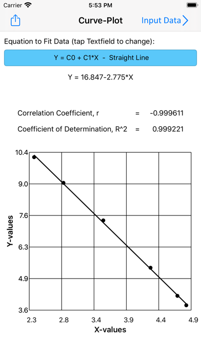
CurveFit uses regression analysis by the method of least squares to find best fit for a set of data to a selected equation.

The curve-fitting technique used in this app is based on regression analysis by the method of least squares. The free version fits a straight line through a data-set using least squares analysis.

One In-App purchase is required to fit the other equations to the data set:
Straight Line : Y = C0 + C1*X (free)
Power Curve : Y = C0 + X^C1 Exponential I : Y = C0 * EXP(C1*X)
Exponential II : Y = C0 * X * EXP(C1*X)
Hyperbolic : Y = (C0 + C1*X)/(1 - C2*X)
Square Root : Y = C0 + C1*SQRT(X)
Polynomial : Y = C0 + C1*X + --- + CN*X^N
Exponential Poly : Y = C0 * EXP(C1*X + --- +
Natural Log : Y = C0 + C1*(LN(X)) + --- +
Reciprocal : Y = C0 + C1/X + --- + CN/X^N

Most literature deals with least squares analysis for straight lines, 2nd degree polynomials, and functions that can be linearized. The input-data is transformed into a format that the can be put into linear forms with undetermined constants. These types of equations are applicable for least-squares regression.

The regression routine is needed for determining values for the set of unknown quantities C1, C2,- - - ,Cm in the equation:

Y = C1 x F1(X) + C2 x F2(X) + - - - + Cm x Fm(X)

The constants are determined to minimize the sum of squares of the differences between the measured values (Y1, Y2, - - - , Yn) and the predicted equation Yc = F(X) which is found by curve-fitting the given data.

The principle of least squares is to find the values for the unknowns C1 through Cm that will minimize the sum of the squares of the residuals:

n
∑(ri) = r12 + r22 + - - - + rn2 = minimum
i=1

This is done by letting the derivative of the above equation equal zero. Thereby there will be generated as many algebraic equations as given data points, and the number of equations will be larger than unknowns.